

Joins form the basis for nearly all data models. Even if you prefer to put all your data in one, very large table - you will still need to join to construct that table.
If you are a frequent Spark user - you might believe that joins are too expensive.
In that case - this blog might be for you.
Because joins are important - we should understand their cost and what tradeoffs a database must make to optimise them. Today, I will take a deeper look at joining in Spark and compare it with its sibling: Databricks Photon.
Configuration
I have spun up two different configuration in Databricks on AWS:
| Cluster | Nodes | Config | DBU/h |
|---|---|---|---|
| Spark | 4 workers in i3.4xlarge | 18.2, Spark 4.1.0, Photon DISABLED | ~20 |
| Photon SQL Warehouse | Small | Serverless SQL Warehouse | ~12 |
According to this doc (kindly pointed out to me by Sergey Pustovich) the "Small" is a 4 worker i3.4xlarge or something equivalent:
However, running this clever tool from Joe Harris indicates that "Databricks Small" might be an ARM system.
In terms of pricing, the two setups are roughly equal. The Spark cluster is probably a bit more powerful than the Photon Serverless Warehouse. But, for our investigation today - being in the same ballpark is good enough.
I have a Delta storage TPC-DS loaded with a scale factor 1000.
Configuration details:
- Largest table:
store_sales- Roughly 600-700GB of data (pre-compression).
- 2.8B rows.
- All surrogate keys in the data model are 8 byte
BIGINTtypes. - Execute
SET use_cached_result = false;on SQL Warehouse make sure repeated runs don't return cached results. - Use a SQL notebook to execute against the raw Spark cluster.
- All queries are run 3 times and we take the fastest runtime (to make sure we have warm disk caches).
- All tables have been fully analysed
- Same catalog is used for Spark and the SQL Warehouse.
Side Note: Spinning up the Raw Spark compute took me around 10 minutes before I got the instances needed (using spot).
On the other hand, Databricks serverless gave me my SQL Warehouse almost immediately - very neat!*
Joining store_sales with item
Our first test query is a join of a small table: item with a large table store_sales. There are 300.000 rows in item and 2.8B rows in store_sales.
First, we inspect the query plan on both Spark and Photon based Databricks. Here is how you do that:
EXPLAIN FORMATTED
SELECT SUM(ss_sales_price)
FROM store_sales F
JOIN item DI ON ss_item_sk = i_item_sk
We get:
Spark:
-----------------------------------------------------------------
AdaptiveSparkPlan (12)
+- == Initial Plan ==
   HashAggregate (11)
   +- Exchange (10)
      +- HashAggregate (9)
         +- Project (8)
            +- BroadcastHashJoin Inner BuildRight (7). <--- JOIN HERE
               :- Project (3)
               :  +- Filter (2)
               :     +- Scan parquet samples.tpcds_sf1000.store_sales (1)
               +- Exchange (6)
                  +- Filter (5)
                     +- Scan parquet samples.tpcds_sf1000.item (4)

Databricks Photon:
-----------------------------------------------------------------
AdaptiveSparkPlan (16)
+- == Initial Plan ==
   ColumnarToRow (15)
   +- PhotonResultStage (14)
      +- PhotonAgg (13)
         +- PhotonShuffleExchangeSource (12)
            +- PhotonShuffleMapStage (11)
               +- PhotonShuffleExchangeSink (10)
                  +- PhotonAgg (9)
                     +- PhotonProject (8)
                        +- PhotonBroadcastHashJoin Inner (7) <--- JOIN HERE
                           :- PhotonProject (2)
                           :  +- PhotonScan parquet samples.tpcds_sf1000.store_sales (1)
                           +- PhotonShuffleExchangeSource (6)
                              +- PhotonShuffleMapStage (5)
                                 +- PhotonShuffleExchangeSink (4)
                                    +- PhotonScan parquet samples.tpcds_sf1000.item (3)
(For the rest of the this blog, I will just show the join parts of the plan for brevity)
We note that both Spark and Photon SQL Warehouse use a "broadcast hash join"
Runtimes:
| Join | Hash Data Size | Spark | Databricks Photon |
|---|---|---|---|
store_sales ⨝ item |
2.4MB | 6.1s | 5.8s |
What's a broadcast join?
The interesting parts of the query plan is this: PhotonBroadcastHashJoin in Databricks and this BroadcastHashJoin in Spark.
For convenience, let us introduce two variables:
B::= The smaller side of the join- Often called the "build"
- In this example, it is
item
P::= The larger side of the join- Often called the "probe".
- In our example, it is
store_sales
A broadcast join runs this following algorithm on a cluster:
- Let all workers create a hash table on a copy of
B. This is the "broadcast" part - as everyone gets their own hash copy. - On each worker, take a share of
Pand use the hash table ofBto emit the join
Exactly how the copy of the hash table gets to all workers in step 1 depends on implementation.
The broadcast join consumes more total memory on the cluster than similar join types - because each node needs a full copy of the hash table. But: it removes the need for shuffling P around the cluster (more about that later).
Joining store_sales with customer
Let's try a bigger join. This time using customer which has 12M rows.
SELECT SUM(ss_sales_price)
FROM store_sales F
JOIN customer DC ON ss_customer_sk = c_customer_sk
The plans are:
Spark:
-----------------------------------------------------------------
SortMergeJoin Inner (10)
:- Sort (5)
:  +- Exchange (4)
:     +- Project (3)
:        +- Filter (2)
:           +- Scan parquet samples.tpcds_sf1000.store_sales (1)
+- Sort (9)
    +- Exchange (8)
        +- Filter (7)
        +- Scan parquet samples.tpcds_sf1000.customer (6)

Databricks Photon:
-----------------------------------------------------------------
PhotonShuffledHashJoin Inner (10)
:- PhotonShuffleExchangeSource (5)
:  +- PhotonShuffleMapStage (4)
:     +- PhotonShuffleExchangeSink (3)
:        +- PhotonProject (2)
:           +- PhotonScan parquet samples.tpcds_sf1000.store_sales (1)
+- PhotonShuffleExchangeSource (9)
    +- PhotonShuffleMapStage (8)
        +- PhotonShuffleExchangeSink (7)
        +- PhotonScan parquet samples.tpcds_sf1000.customer (6)
Here, we start to see a significant difference between Photon and Spark:
| Join | Hash Data Size | Spark | Databricks Photon |
|---|---|---|---|
store_sales ⨝ item |
2.4MB | 6s | 5.8s |
store_sales ⨝ customer |
96MB | 38s | 8.7s |
What's Sort/Merge Join?
What does the SortMergeJoin in the Spark query plan mean?
Sort/Merge is a "classic join" that has been used throughout history.
The algorithm is:
- Partition both
PandBusing a hash or range of the join key - "Shuffle" both
PandBaround the cluster- Each worker in the cluster receives equals portion of the data
- Because we have partitioned the data, the join keys on each worker are guaranteed not to overlap
- This operation is sometimes called "exchange" (as we see in the Spark query plan)
- This involves a lot of network traffic - it's expensive
- Each worker sorts it own partitions of
BandP- On large joins, this will spill data to disk
- The sort is also of time complexity: O(|B|*log(|B|)+|P|+log(|P|))
- Each worker merges the sorted streams of its local
PandBand emits the result.
Variations of this algorithm exist which interleave the sorting, merging and shuffling. But the important takeaway here is: Sort/Merge join requires both side of the join to be sorted and shuffled.
The sort/merge join is good when memory is scarce and CPUs are old - such as when running on a old mainframe. It can also be the superior join strategy if one side of the join is already sorted on the join key or if both sides of the join are gigantic compared to the total amount of cluster memory (rare these days).
But in most cases - including the one we are seeing here - Sort/Merge is just a bad join algorithm. Sorting and merging interact very poorly with the CPUs branch predictor and has terrible behaviour in terms of memory access patterns.
Sort Merge doesn't scale
The problem with Sort/Merge gets worse when queries have many joins.
You now have to sort the large table (P) multiple times - once per join. This is an expensive operation on a large dataset.
We can see this effect by executing a more complex query. If we compare 1 and 2 joins and add some additional payload (common in analytical systems) we begin to see why sort/merge is so bad.
Fortunately, customer_demographicsin TPC-DS is perfect for this test, because it can join twice to store_sales:
SELECT SUM(ss_sales_price),
  SUM(ss_net_paid),
  SUM(ss_ext_discount_amt),
  SUM(ss_ext_tax),
  SUM(ss_coupon_amt),
  SUM(ss_ext_wholesale_cost),
  SUM(ss_net_profit),
  SUM(ss_list_price),
  SUM(ss_quantity),
  MAX(DD1.cd_education_status)
-- Add for 2 joins
-- , MAX(DD2.cd_education_status)
FROM samples.tpcds_sf1000.store_sales F
JOIN samples.tpcds_sf1000.customer_demographics DD1 ON ss_cdemo_sk = DD1.cd_demo_sk
-- Add for 2 joins
--JOIN samples.tpcds_sf1000.customer_demographics DD2 ON ss_hdemo_sk = DD2.cd_demo_sk
The dramatic effect of sort/merge on queries with more joins is now obvious:
| Query | Spark | Photon | Sort/Merge Penalty |
|---|---|---|---|
| 1 join | 119s | 23s | 5.2x |
| 2 joins | 518s | 27s | 19.2x |
Photon to the Rescue: What's a Shuffle Hash Join?
Notice that Databricks Photon picks a PhotonShuffledHashJoin when joining customer with store_sales.
The algorithm for a shuffle hash is:
- Partition both
PandBusing a hash of the join key - "Shuffle" both
PandBaround the cluster- So far, same as sort/merge
- Same network overhead
- Each worker builds a hash table over the partitions of
Bit owns- Since the data is partitioned, we can effective utilise the memory of the entire cluster for this (no copies like the broadcast)
- Each worker looks up data from the
Pinto the local hash table ofBand emits the result
As we can clearly see, this join is much faster than sort/merge and has a lower time complexity of only O(|B|+|P|). But it still requires both sides of the join to be shuffled - consuming significant network traffic.
Even though our customer table is only 96MB and we 122GB (i.e. 1500x more) memory on each node - the optimiser still picks shuffle hash.
Side Note: There exists an optimisation of the shuffle hash which does not require the resulting hash table to fit in memory. This is called "grace hash" and is best explained by the man himself, Andy Pavlo:
- CMU: Hash Joins, Sort-Merge Joins, Nested Loop Join Algorithms (around the 55 minute mark)
On my small (1TB) dataset, I was not able to force Databricks to do perform Sort/Merge - it stuck to Shuffle Hash even when doing the much larger join of store_sales with store_returns. I also tried a large join on an 2xSmall system - with no luck: Databricks loves its Shuffle hash.
Side Note: Curious to know from readers if there is a way to get sort/merge out of Databricks with an equi join. Ping me on LinkedIn if you have some ideas.
Join strategies summary
This table can hopefully help you think about the tradeoffs that database must consider when picking a distributed join strategy:
| Distribute Join | Cluster Memory | Network | Shuffle | Time Complexity |
|---|---|---|---|---|
| Broadcast | High | Low | B | O(|B|+|P|) |
| Shuffle Hash | Low | High | B and P | O(|B|+|P|) |
| Sort/Merge | Low | High | B and P | O(|B|*log(|B|)+|P|*log(|P|)) |
The tradeoff can be summarised as: "Sacrifice a bit of memory to save a lot of network and gain a lot of speed"
Databricks Adaptive joining - Clever
Remember I said that Photon shuffle hash still needs to move data around the cluster between workers? It turns out that Photon is clever about this. While executing, it realises that it does not need to do that (Because B is pretty small).
The runtime plan can be found under Query History tab in Databricks, and it is:
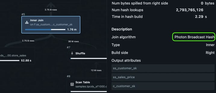
Notice that even though EXPLAIN expected a shuffle hash, Databricks chose (wisely) to execute a broadcast.
However, we can coerce Databricks into a shuffle hash by adding payload to the small side of the join. The column c_email_address has an average size of 27 bytes. If we ask for that column in the query result, it increase the size of the hash table needed to join (to 400MB of data)
This query does the trick:
SELECT SUM(ss_sales_price),
  MAX(c_email_address). -- Payload, make the join bigger
FROM store_sales F
JOIN customer DC ON ss_customer_sk = c_customer_sk;
Inspecting the actual plan in Query History, we are now getting a shuffle hash - even at runtime. The impact is dramatic:
| Join | Hash Data Size | Spark | Databricks Photon |
|---|---|---|---|
store_sales ⨝ item |
2.4MB | 6.1s | 5.8s |
store_sales ⨝ customer |
96MB | 38s | 8.7s |
store_sales ⨝ customer (payload) |
400MB | 53s | 20s |
Switching to a shuffle join more than doubles execution time, even on Photon. Notice that Photon is still outrunning a vanilla Spark which relies on sort/merge for the same query.
We only needed 400MB of memory (out of the 122GB we have) on each worker to do a broadcast. Yet, neither Spark nor Photons query optimiser decided to do it.
Forcing the Broadcast
Fortunately, there are ways to tell the optimiser: "Trust me, I'm a pro".
The following works on both Databricks and vanilla Spark (see Spark Hints)
SELECT /*+ BROADCAST(DC) */
  SUM(ss_sales_price),
  MAX(c_email_address). -- Payload, make the join bigger
FROM store_sales F
JOIN customer DC ON ss_customer_sk = c_customer_sk;
Our knowledge pays off, gaining us 1.5x improvement in runtime and a large reduction in network traffic:
| Join | Hash Data Size | Spark | Databricks Photon |
|---|---|---|---|
store_sales ⨝ item |
2.4MB | 6.1s | 5.8s |
store_sales ⨝ customer |
96MB | 38s | 8.7s |
store_sales ⨝ customer (payload) |
400MB | 53s | 20s |
store_sales ⨝ customer (payload+broadcast) |
400MB | 30s | 13s |
The effect is even stronger if we force broadcast on Spark for our previous 1 and 2 join test:
| Query | Spark Sort/Merge | Spark Broadcast | Photon | Sort/Merge | Broadcast |
|---|---|---|---|---|---|
| 1 join | 119s | 48s | 23s | 5.2x | 2x |
| 2 joins | 518s | 54s | 27s | 19.2x | 2x |
Using broadcast on Spark makes multiple joins scalable again!
Unless you force it - scalable joins is not the behaviour you are going to get on Spark in its default configuration.
Side Note: You can globally control when Spark decides to use Broadcast joins with. See this resource Automatically Broadcasting Joins.
Fascinatingly, the default threshold is only 10MB on each worker - and this appears to be the same default used by the Spark installed by Databricks
Forcing Spark to do Shuffle Hash
It turns out that Spark can also do Shuffle Hash but it is conservative about picking this strategy.
Here is how you force shuffle hash:
SELECT /*+ SHUFFLE_HASH(DC, F) */  SUM(ss_sales_price), MAX(c_email_address)
FROM samples.tpcds_sf1000.store_sales F
JOIN samples.tpcds_sf1000.customer DC ON ss_customer_sk = c_customer_sk;
And here are the results:
| Join | Hash Data Size | Spark | Databricks Photon |
|---|---|---|---|
store_sales ⨝ customer (default) |
96MB | 38s | 8.7s |
store_sales ⨝ customer (shuffle) |
96MB | 32s | - |
store_sales ⨝ customer (payload) |
400MB | 53s | 20s |
store_sales ⨝ customer (payload+broadcast) |
400MB | 30s | 13s |
store_sales ⨝ customer (payload+shuffle) |
400MB | 45s | - |
Another case of the human beating the optimiser.
Why Spark does not pick shuffle hash more often is a mystery to me. Shuffle Hash, when you cannot broadcast, is generally considered the superior join strategy.
Conclusions
Today, we have seen how the join strategy you pick matters a lot - particularly in a distributed system.
- When you have the memory - Pick Broadcast join and save your network!
- Avoid Sort/merge (Spark's default) for nearly all cases
- If low on memory, pick shuffle hash
- Particularly if your database engine implements grace hash join
- Databricks Photon does wonders for you here
- You can control join strategies on Spark and Databricks with hints
- Databricks appears very conservative about memory - forcing broadcast is sometimes worth it
- Spark's default configuration is likely not the one you want - unless you are running on very low memory systems (ex: using a Rasperry Pi as the scale node)
Here at Floe, we are building a new database engine for the cloud. One that will make better query plans and use modern hardware they way it was designed to be used.
Follows us in the link above to stay updated with our development.
Thought: Are Spark Joins actually expensive?
In my interactions on LinkedIn - I have often wondered why it is widely believed that "joins are expensive". In particular, this appears to be a common view held by Spark users.
I now have a hypothesis...
Is it perhaps the case that some Spark users have grown up in a world of default configurations? Even on large clusters? If your Spark cluster is configured to do sort/merge joins for inputs bigger than 10MB - then joining is going to be a very painful experience for you.
This could lead you to (wrongly) conclude that modern compute and storage is better off with highly denormalised data models. Because Spark, with its love of Sort/Merge join, might have taught you that "joins are expensive".
The conclusion to draw from your sort/merge trauma is not "joins are expensive". Instead, a better takeaway would be: "you probably need to configure your cluster to use the memory you actually have".