
Geo joins look innocent:
SELECT *
FROM A
JOIN B
  ON ST_Intersects(A.geo, B.geo);
…but at scale they can become the query that ruins your day.
Geospatial functions are expensive, and they often force a loop join that starts to feel quadratic as your tables grow.
The core idea in this post is simple: we’ll see how Floe automatically rewrites this kind of query and takes advantage of H3 indexes for dramatic speedup.
What’s a geo join
A geo join is any join whose ON clause is a spatial predicate:
ST_IntersectsST_CoversST_DWithin- ...
A canonical example:
SELECT *
FROM A
JOIN B
  ON ST_Intersects(A.geo, B.geo);
Why it hurts at scale
Modern databases make joins fast by turning them into hash joins over keys. If you can hash-partition both inputs on the join key, each worker compares only its share instead of comparing everything to everything. If the data is nicely distributed, this decreases the complexity from quadratic to linear.
Spatial predicates don’t give you a clean join key. So you end up in a terrible situation:
- you have to compare every value with each other (the quadratic complexity)
- plus an expensive predicate on each candidate pair
That’s the situation we want to escape.
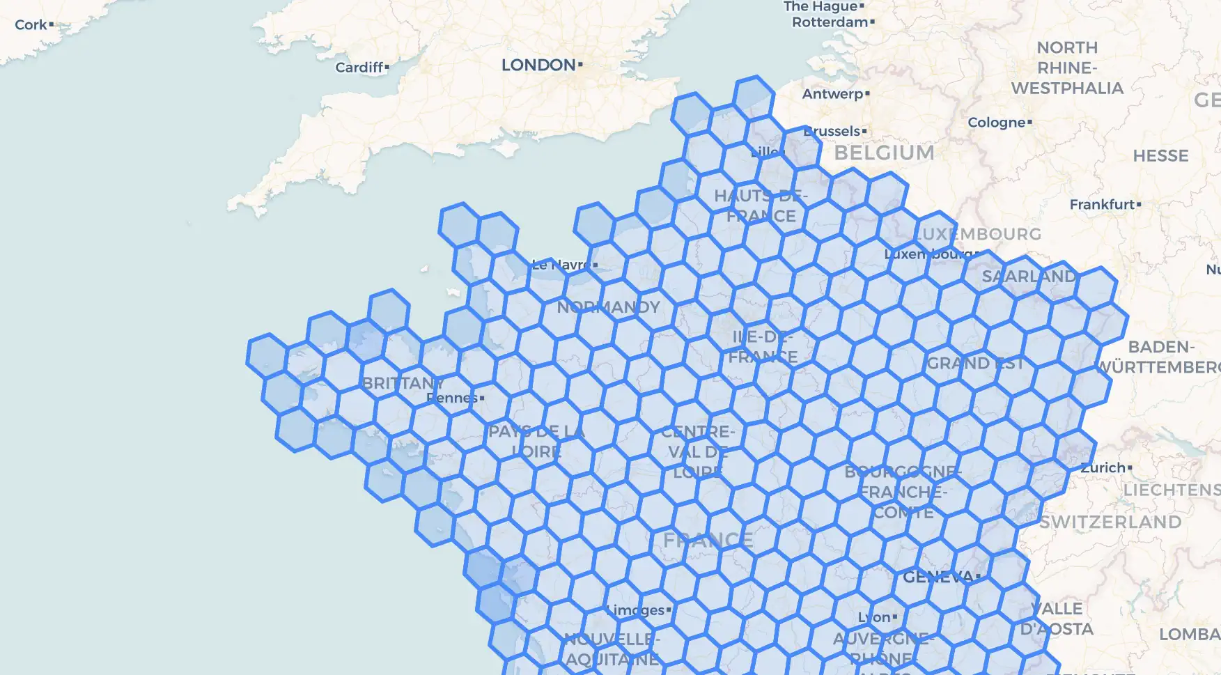
Meet H3
H3 (originally from Uber) partitions the Earth into a hierarchy of mostly hexagonal cells.

Two properties matter for us:
- Hierarchical resolution: you choose a resolution from coarse to fine.
- Compact keys: each cell is a
BIGINT, so it behaves like a normal join key: hashable, sortable, distributable.
Most importantly, it lets us represent a geography as a set of cell IDs that covers it.
If two shapes intersect, then their H3 cover sets share at least one cell.
That gives us a path to rewrite “do these shapes intersect?” into “do these two sets overlap?” which a database can execute as a plain equi-join.

Conservative approximation (false positives only)
Cell coverage is an approximation of the exact geometry:
- It’s OK to keep extra candidates (false positives): they’ll be removed by the exact predicate.
- It’s not OK to miss true matches (false negatives): if we drop them in the pre-filter, no later step can recover them.
So we generate coverage so it over-approximates the shape (the coverage contains the shape).
From geography predicate to set-ops
The rewrite: exact join → fast filter + exact recheck
Baseline:
SELECT *
FROM A
JOIN B
  ON ST_Intersects(A.geo, B.geo);
With H3, the planner inserts a filtering phase:
- Generate H3 coverage for
A - Generate H3 coverage for
B - Join on
cell(fast integer equi-join) - Deduplicate candidates (the same pair can match on multiple cells)
- Run the exact predicate on candidates only
A concrete template:
WITH
  a_cells AS (
    SELECT
      a.id,
      a.geo,
      c.cell
    FROM A a
    JOIN h3_coverage(a.geo, /* resolution */ 3, /* full cover */ true) c
      ON TRUE
  ),
  b_cells AS (
    SELECT
      b.id,
      b.geo,
      c.cell
    FROM B b
    JOIN h3_coverage(b.geo, 3, true) c
      ON TRUE
  ),
  candidates AS (
    SELECT DISTINCT
      a_cells.id  AS a_id,
      a_cells.geo AS a_geo,
      b_cells.id  AS b_id,
      b_cells.geo AS b_geo
    FROM a_cells
    JOIN b_cells USING (cell)
  )
SELECT *
FROM candidates
WHERE ST_Intersects(a_geo, b_geo);
What the database gets “for free”
With this rewrite, the heavy work becomes an equi-join on (cell):
- It’s an integer join → hashing is cheap.
- It’s naturally distributable → you can hash-partition on
cellacross workers. - The expensive predicate becomes a cleanup step instead of the main event.
Three questions readers always ask
“Isn’t that approximate?” Yes — the H3 step is an approximation used as a pre-filter. Correctness is preserved by the final exact predicate recheck.
“Won’t that create false positives?” Yes, and that’s expected. The goal is to reduce the candidate set enough that exact checks become cheap.
“How do I pick a resolution?” Resolution is the tradeoff knob: higher resolution usually reduces false positives but increases the number of cells generated per shape. (We’ll cover how to measure and choose this in the Numbers section later.)
See the effect
When a user enters a simple query to join countries with the cities they contain, the planner automatically applies the rewrite:
EXPLAIN ANALYZE SELECT * FROM world_cities JOIN countries ON ST_Intersects(world_cities.geo, countries.geo);
>>>
Planning time: 2.291 ms
rows_actual    node
     142141    SELECT
     142141    FILTER WHERE ST_INTERSECTS(MAX(MAX(world_cities.geo)), MAX(MAX(countries.geo)))
                 geojoin filtered rows ratio: 99.62%
     199848    GROUP BY (countries.rowunique, world_cities.rowunique)
     199848    DISTRIBUTE ON HASH(world_cities.rowunique),HASH(countries.rowunique))
     199848    GROUP BY PARTIAL (countries.rowunique, world_cities.rowunique)
     224075    INNER HASH JOIN ON (COALESCE(h3_coverage_geodesic.h3_coverage_geodesic , $1 , const )  = COALESCE(h3_coverage_geodesic.h3_coverage_geodesic , $0 , const ) )
     147043    |-DISTRIBUTE ON HASH(COALESCE(h3_coverage_geodesic.h3_coverage_geodesic , $0 , const ) )
     147043    | LEFT OUTER FUNCTION JOIN H3_COVERAGE_GEODESIC(world_cities.geo, 3, t, t) ON true
     147043    | SCAN world_cities
      17223    |-BUILD HASH
      17223      DISTRIBUTE ON HASH(COALESCE(h3_coverage_geodesic.h3_coverage_geodesic , $1 , const ) )
      17223      LEFT OUTER FUNCTION JOIN H3_COVERAGE_GEODESIC(countries.geo, 3, t, t) ON true
        256      SCAN countries

142141 rows returned
Read: 16.92MiB, Distributed: 5.85GiB, Network: 8.00GiB
Database: yellowbrick_test_utf8
Execution time: 1220.118 ms, End time: 2025-12-16 14:00:50
Without the rewrite, the join would face ~`256 * 147043 = 37.6 million` country×city pairs.
Instead, we’re doing 199848 calls to ST_Intersects, of which we keep 142141 pairs, a 99.6% reduction.
On-the-fly indexing
A possible approach is to materialize an index table (row_id → list of H3 cells) and maintain it. This avoids the somewhat expensive step of computing H3 indexes.
We chose a different route: compute coverage at query time as part of the rewrite
Why it’s practical:
- Works over views, CTEs and subqueries, not just base tables.
- Avoids extra storage and index maintenance.
- Keeps experimentation easy (resolution, coverage mode, predicate type).
This makes it easy to play with data cleaning directly in the query:
with cleaned_cities as
    (select distinct st_reduceprecision(geo, 100) geo from world_cities) -- Dedup cities that are less than 100 meters apart
select count(*) from countries join cleaned_cities on st_intersects(countries.geo, cleaned_cities.geo);
Numbers
Let’s look at some numbers.
We’ll use a join between 256 polygons representing countries and points representing world cities:
SELECT *
FROM world_cities
JOIN countries
  ON ST_Intersects(world_cities.geo, countries.geo);
In this dataset, countries.geo is a polygon or multipolygon with 418 vertices on average.
We ran these tests on a cluster with 15 workers, each with a Xeon E5-2695 (16 cores @ 2.10GHz) and 1 TB of memory.
First, let’s look at the effect of H3 resolution.
Each time we increase the resolution by 1, the average size of a cell decreases by ~6×.
- Baseline is the time the query takes without H3 indexing. (459 seconds)
- GeoJoin is the time the query takes with the rewrite.
The GeoJoin time follows a U-shape:
- Increasing the resolution improves row rejection.
- Increasing it too much makes indexing and the
(cell)join too expensive.
At best, at resolution 3, the geo join takes 1.17 seconds — a 400× improvement.
We can also see where the time goes:
- At low resolution it’s really fast to index both tables — less than 10% of the time at resolution 2.
- But it increases rapidly after resolution 4.
And even when we eliminate indexing time, at high resolution there are so many rows in the join that the geo join time starts to increase.
| Resolution | Baseline query Time (s) | GeoJoin Time (s) | Speedup | Index countries Time (s) | Index cities Time (s) | Total indexing Time (s) | GeoJoin - Index Time (s) | Index Time / GeoJoin Time | Average Hexagon Area (km2) |
|---|---|---|---|---|---|---|---|---|---|
| 0 | 459.7 | 16.2 | 28.3 | 0.2 | 0.03 | 0.2 | 16.0 | 0.0 | 4,357,449 |
| 1 | 459.7 | 3.0 | 152.7 | 0.1 | 0.0 | 0.1 | 2.9 | 0.0 | 609,788 |
| 2 | 459.7 | 1.4 | 338.8 | 0.1 | 0.0 | 0.1 | 1.2 | 0.1 | 86,801 |
| 3 | 459.7 | 1.1 | 392.5 | 0.3 | 0.0 | 0.3 | 0.9 | 0.3 | 12,393 |
| 4 | 459.7 | 2.2 | 205.0 | 1.4 | 0.0 | 1.4 | 0.9 | 0.6 | 1,770 |
| 5 | 459.7 | 13.2 | 34.8 | 8.2 | 0.0 | 8.3 | 4.9 | 0.6 | 252 |

Conclusion
By rewriting spatial predicates into set operations on H3 cells, we let the database do what it’s best at: parallel hash joins on compact keys. This leads to a dramatic speedup of geography operations.
We could improve these results even more by avoiding calls to the geography predicate in trivial-true cases. For instance, when a point lies well inside a large polygon.